Kalmann Filters on a 32 Kb Microcontroller
In my fourth year, I took the now-defunct 4B25
module on embedded systems. The professor is an
industry powerhouse, and he had high standards. He gave us an FRDM-KL03
development board so small that even #include <cmath>
didn't link. The goal was to produce an uncertainty aware measurement of
the orientation of the board. This was quite a fun challenge that I
still look fondly on today.
Mathematical Background
The core idea is that we measure a noisy estimate of the acceleration \(\mathbf{\hat a}_t\), and we want to infer the roll angle of the system at that time \(\phi_t\). There is some process \( A \) that governs how \(\phi_t \) is related to \( \phi_{t+1} \), and a different process \(B\) that governs the measurement of \(\mathbf{\hat a}_t\) from \(\phi_t\). This formulation gets us our familiar state space model:
\[ \begin{array}{ccccccc} \boxed{~ \phi_{t-1} ~} & \xrightarrow{\;\normalsize A\;} & \boxed{~ \phi_t ~} & \xrightarrow{\;\normalsize A\;} & \boxed{~ \phi_{t+1} ~} & \xrightarrow{\;\normalsize A\;} & \boxed{~ \phi_{t+2} ~} \\ \Big\downarrow B && \Big\downarrow B && \Big\downarrow B && \Big\downarrow B \\ \boxed{~ \mathbf{\hat a}_{t-1} ~} && \boxed{~ \mathbf{\hat a}_t ~} && \boxed{~ \mathbf{\hat a}_{t+1} ~} && \boxed{~ \mathbf{\hat a}_{t+2} ~} \end{array} \]Deriving the Latent Process \(A\)
How \( \phi_t\) becomes \( \phi_{t+1}\) is intimately coupled with how we discretize the system into timesteps of width \(\Delta t\). We assume that the roll velocity, \( \dot{\phi}_t\), is a Gaussian random walk, and \(\phi_t \) is defined from this:
\[ \phi_{t+1} = \phi_t + \Delta t\,\dot{\phi}_t, \qquad \dot{\phi}_{t+1} \sim \mathcal{N} \left(\dot{\phi}_t,\; \Delta t\,\sigma_{\dot{\phi}}^2\right) \]With a little bit of algebra, you can represent this in state-space form to fully specify the process:
\[ \begin{pmatrix} \phi_{t+1} \\ \dot{\phi}_{t+1} \end{pmatrix} \sim \mathcal{N}\left( \begin{pmatrix}1 & \Delta t \\ 0 & 1\end{pmatrix} \begin{pmatrix}\phi_t \\ \dot{\phi}_t\end{pmatrix}, \; \sigma_{\dot{\phi}}^2 \left( \begin{matrix} {\Delta t^3}/{3} & {\Delta t^2}/{2} \\ {\Delta t^2}/{2} & \Delta t \end{matrix} \right) \right) \]Deriving the Observation Process \(B\)
You can show that Gaussian component-wise observation noise in the vector acceleration reading \(\mathbf{ \hat a}_t \) approximately leads to a Gaussian posterior. This can be expressed as
\[ \hat\phi_{t} \sim \mathcal{N}\left( \begin{pmatrix}1 & 0 \end{pmatrix} \begin{pmatrix}\phi_t \\ \dot{\phi}_t\end{pmatrix}, \; \frac{\sigma_a^2}{g\lvert\mathbf{\hat a}_t\rvert} \right) \]where the variance is inversely proportional to the magnitude of the measurement reading.
Kalmann filtering for the orientation, \(p(\phi_t \mid \{\mathbf{ \hat a_i}\}^{t}_{0} ) \)
In state space form, solving for the estimate is straightforward. Just copy the Kalmann filtering equations from a textbook
\[ \begin{aligned} P_{t|t-1} &= \Sigma_v + A,P_{t-1|t-1},A^T \\ K_t &= P_{t|t-1} B^T \left(B P_{t|t-1} B^T + \Sigma_w\right)^{-1} \\ \mu_{t|t} &= A,\mu_{t-1|t-1} + K_t\left(y_t - B A,\mu_{t-1|t-1}\right) \\ P_{t|t} &= (I - K_t B),P_{t|t-1} \\ \end{aligned} \]
and substitute
\[ \begin{aligned} P_{t|t-1} &= \sigma_{\dot{\phi}}^2 {\begin{pmatrix} {\Delta t^3}/{3} & {\Delta t^2}/{2} \\ {\Delta t^2}/{2} & \Delta t \end{pmatrix}} + {\begin{pmatrix}1 & \Delta t \\ 0 & 1\end{pmatrix}}P_{t-1|t-1}{\begin{pmatrix}1 & \Delta t \\ 0 & 1\end{pmatrix}}^T \\ K_t &= P_{t|t-1} {\begin{pmatrix}1 & 0 \end{pmatrix}}^T \left({\begin{pmatrix}1 & 0 \end{pmatrix}} P_{t|t-1} {\begin{pmatrix}1 & 0 \end{pmatrix}}^T + \frac{\sigma_a^2}{g\lvert\mathbf{\hat a}_t\rvert} \right)^{-1} \\ \mu_{t|t} &= {\begin{pmatrix}1 & \Delta t \\ 0 & 1\end{pmatrix}}\mu_{t-1|t-1} + K_t\left(y_t - {\begin{pmatrix}1 & 0 \end{pmatrix}} {\begin{pmatrix}1 & \Delta t \\ 0 & 1\end{pmatrix}}\mu_{t-1|t-1}\right) \\ P_{t|t} &= (I - K_t {\begin{pmatrix}1 & 0 \end{pmatrix}})P_{t|t-1} \end{aligned} \]
This is visually alot of math, but it translates identically into four lines of neat Python:
P_pred = Sigma_v + A @ P @ A .T
K = P_pred @ B .T / (B @ P_pred @ B .T + Sigma_w )
mu = A @ mu + K * (y_t - B @ A @ mu )
P = (I_2 - K @ B ) @ P_pred
On a 32 kB Microcontroller?
I need to write the above in C. If I'd have done this coursework in the era of LLMs, I could have easily cranked out a fixed-size matrix math library for my exact use case. Fortunately, I did a little more thinking and found quite an interesting optimization.
See, there's a lot of problem-specific optimizations we miss out on with a standard 2x2 matrix multiplication library:
- Symmetric matrices (eg. \(P_{t|t}\) and \(P_{t|t-1}\)) could be calculated and represented more efficiently
- Matrices with \(1\) and \(0\) elements use more floating point operations than strictly necessary
If you get a computer to do the algebra for you, it can expand out all of the terms in the matrices you're calculating, so you can avoid writing your own matrix library all together:
mu_t1 = dt * mu2 + mu1 + 3 * (- dt * mu2 - mu1 + y_t )* (dt ** 3 * sv / 3 + dt * p12 + dt * (dt * p22 + p12 ) + p11 )/ (dt ** 3 * sv + 3 * dt ** 2 * p22 + 6 * dt * p12 + 3 * p11 + 3 * sw )
mu_t2 = mu2 + 3 * (- dt * mu2 - mu1 + y_t )* (dt ** 2 * sv / 2 + dt * p22 + p12 )/ (dt ** 3 * sv + 3 * dt ** 2 * p22 + 6 * dt * p12 + 3 * p11 + 3 * sw )
p_t11 = (- 3 * (dt ** 3 * sv / 3 + dt * p12 + dt * (dt * p22 + p12 ) + p11 )/ (dt ** 3 * sv + 3 * dt ** 2 * p22 + 6 * dt * p12 + 3 * p11 + 3 * sw ) + 1 ) * (dt ** 3 * sv / 3 + dt * p12 + dt * (dt * p22 + p12 ) + p11 )
p_t12 = (- 3 * (dt ** 3 * sv / 3 + dt * p12 + dt * (dt * p22 + p12 ) + p11 )/ (dt ** 3 * sv + 3 * dt ** 2 * p22 + 6 * dt * p12 + 3 * p11 + 3 * sw ) + 1 )* (dt ** 2 * sv / 2 + dt * p22 + p12 )
p_t21 = dt ** 2 * sv / 2 + dt * p22 + p12 - 3 * (dt ** 2 * sv / 2 + dt * p22 + p12 )* (dt ** 3 * sv / 3 + dt * p12 + dt * (dt * p22 + p12 ) + p11 )/ (dt ** 3 * sv + 3 * dt ** 2 * p22 + 6 * dt * p12 + 3 * p11 + 3 * sw )
p_t22 = dt * sv + p22 - 3 * (dt ** 2 * sv / 2 + dt * p22 + p12 )** 2 / (dt ** 3 * sv + 3 * dt ** 2 * p22 + 6 * dt * p12 + 3 * p11 + 3 * sw )])
This is already good enough to ship. Writing the above in C, the
compiler produces 200 instructions by default and just ~70 instructions
when compiling with -O3 -ffast-math. Here's what godbolt
says:
Alot of this is achieved by deduplicating common subexpressions, eg.
by noticing that we calculate dt**2*sv many times, and
storing the result in a register.
Can we do better?
Beating The Compiler
Now that we're using computer algebra software for algebraic expansion, lets exercise it a little more. Why not try to do the common subexpression elimination directly in CAS, rather than in the C compiler? This is roughly the code I used for it:
from sympy import Symbol , Matrix , cse , eye
# compile time parameters
dt , sv , sw = Symbol ("dt" ), Symbol ("sv" ), Symbol ("sw" )
A = Matrix ([[1 , dt ], [0 , 1 ]])
B = Matrix ([[1 , 0 ]])
Sigma_v = sv * Matrix ([[0 , dt ** 2 / 2 ], [dt ** 2 / 2 , dt ]])
Sigma_w = Matrix ([[sw ]])
# runtime time variables
mu1 , mu2 , p11 , p12 , p22 = Symbol ("mu1" ), Symbol ("mu2" ), Symbol ("p11" ), Symbol ("p12" ), Symbol ("p22" )
mu = Matrix ([mu1 , mu2 ])
P = Matrix ([[p11 , p12 ], [p12 , p22 ]])
# propagation logic
P_pred = Sigma_v + A * P * A .T
K = P_pred * B .T * (B * P_pred * B .T + Sigma_w ).inv ()
y = Matrix ([Symbol ("y" )])
mu_t = A * mu + K * (y - B * A * mu )
P_t = (eye (2 ) - K * B ) * P_pred
# CAS query
print (* cse ([mu_t , P_t ]), sep = "\n" )
and the output is kindof like this:
x0  = dt * mu2 + mu1
x1  = -x0 + y_t
x2  = dt * p12
x3  = dt**3 * sv
x4  = dt * p22 + p12
x5  = dt * x4 + p11 + x2 + x3 / 3
x6  = dt**2
x7  = 3 / (3 * p11 + 3 * p22 * x6 + 3 * sw + 6 * x2 + x3)
x8  = x5 * x7
x9  = sv * x6 / 2 + x4
x10 = 1 - x8

mu_t = [[    x0 + x1*x8],
        [mu2 + x1*x7*x9]]

P_t =  [[     x10*x5,                 x10*x9],
        [-x8*x9 + x9, dt*sv + p22 - x7*x9**2]]
Not only did I compile this, but I also compiled a variant of this
where I assumed that dt**3 is approximately zero. Here's
what Godbolt says about our new code:
Comparing the Implementations
It's super interesting to see that there is still room for alternate
mathematical optimizations, even with -O3 -ffast-math.
| Naive | CSE | CSE + assume \(dt^3 \approx 0\) | |
|---|---|---|---|
| Instruction Count (GCC) | 69 | 59 | 54 |
| Instruction Count (ARM Clang) | 61 | 57 | 47 |
I find it tricky to properly dig into the resulting assembly and unpack why the compiler misses optimizations, but I suspect compiler optimizations aren't allowed to restructure an expression graph globally?
I suspect that restructuring a global expression graph is a kind of unboundedly tricky problem, with solutions in this space creating and exploiting clever redundancies to minimize the combinatorial explosion of possibilities.
That's all folks
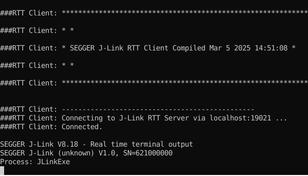
In case you're curious, here's what the TUI (written in raw C!) looked like: